
It was just announced that this year's Nobel Prize in physics goes to Takaaki Kajita from the Super-Kamiokande Collaboration and Arthur B. McDonald from the Sudbury Neutrino Observatory (SNO) Collaboration “for the discovery of neutrino oscillations, which shows that neutrinos have mass.” On this occasion, I am reposting a brief summary of the evidence for neutrino masses that I wrote in 2007.
Neutrinos come in three known flavors. These flavors correspond to the three charged leptons, the electron, the muon and the tau. The neutrino flavors can change during the neutrino's travel, and one flavor can be converted into another. This happens periodically. The neutrino flavor oscillations have a certain wavelength, and an amplitude which sets the probability of the change to happen. The amplitude is usually quantified in a mixing angle θ. In this, sin2(2 θ) = 1, or θ = π/4 corresponds to maximal mixing, which means one flavor changes completely into another, and then back.
This neutrino mixing happens when the mass-eigenstates of the Hamiltonian are not the same as the flavor eigenstates. The wavelength λ of the oscillation turns out to depend (in the relativistic limit) on the difference in the squared masses Δm2 (not the square of the difference!) and the neutrino's energy E as λ = 4E/Δm2. The larger the energy of the neutrinos the larger the wavelength. For a source with a spectrum of different energies around some mean value, one has a superposition of various wavelengths. On distances larger than the typical oscillation length corresponding to the mean energy, this will average out the oscillation.
The plot below from the KamLAND Collaboration shows an example of an experiment to test neutrino flavor conversion. The KamLAND neutrino sources are several Japanese nuclear reactors that emit electron anti-neutrinos with a very well known energy and power spectrum, that has a mean value around some MeV. The average distance to the reactors is ~180 km. The plot shows the ratio of the observed electron anti-neutrinos to the expected number without oscillations. The KamLAND result is the red dot. The other data points were earlier experiments in other locations that did not find a drop. The dotted line is the best fit to this data.

[Figure: KamLAND Collaboration]
One sees however that there is some kind of redundancy in this fit, since one can shift around the wavelength and stay within the errorbars. These reactor data however are only one of the measurements of neutrino oscillations that have been made during the last decades. There are a lot of other experiments that have measured deficites in the expected solar and atmospheric neutrino flux. Especially important in this regard was the SNO data that confirmed that indeed not only there were less solar electron neutrinos than expected, but that they actually showed up in the detector with a different flavor, and the KamLAND analysis of the energy spectrum that clearly favors oscillation over decay.
The plot below depicts all the currently available data for electron neutrino oscillations, which places the mass-square around 8×10⁻⁵ eV2, and θ at about 33.9° (i.e. the mixing is with high confidence not maximal).
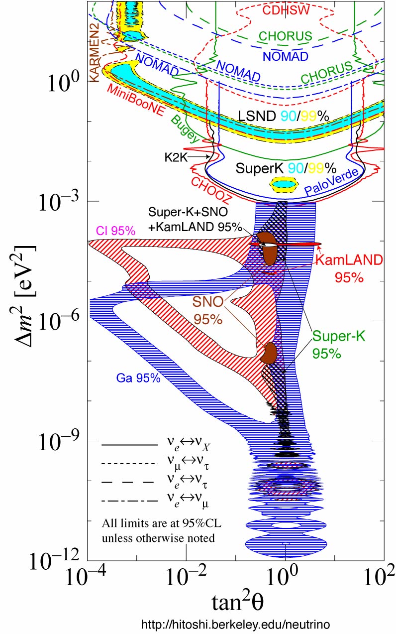
[Figure: Hitoshi Murayama, see here for references on the used data]
The lines on the top indicate excluded regions from earlier experiments, the filled regions are allowed values. You see the KamLAND 95%CL area in red, and SNO in brown. The remaining island in the overlap is pretty much constrained by now. Given that neutrinos are so elusive particles, and this mass scale is incredibly tiny, I am always impressed by the precision of these experiments!
To fit the oscillations between all the known three neutrino flavors, one needs three mixing angles, and two mass differences (the overall mass scale factors out and does not enter, neutrino oscillations thus are not sensitive to the total neutrino masses). All the presently available data has allowed us to tightly constrain the mixing angles and mass squares. The only outsider (that was thus excluded from the global fits) is famously LSND (see also the above plot), so MiniBooNE was designed to check on their results. For more info on MiniBooNE, see Heather Ray's excellent post at CV.
This post originally appeared in December 2007 as part of our advent calendar A Plottl A Day.
...masses and angles....
ReplyDeleteThanks, fixed that...
ReplyDeleteIt won't steal the show from a Nobel but I noticed the blogger recently won 1st prize in a prestigious essay context (steering the future) that pays a substantial cash prize. I took in your essay and it's really good and I can see what they saw in it when judging. You could probably land yourself a good commercial role on the strength of that (and all the other things you've got). It's difficult saying all this without coming over like pompous twit, so what the hell, I'll finish with "well done"!
ReplyDelete